Analog Computers
Abstract
Before the digital computer won, the fastest way to solve a hard equation was to build a physical model of it. Analog computers represent numbers as continuous quantities, the angle of a shaft, the voltage on a wire, and compute by letting the physics do the arithmetic. They predicted tides, aimed anti-aircraft guns, guided the V-2 rocket, and flew the simulations that designed the Apollo program. Then digital machines caught up on speed and passed them on precision and programmability, and by the 1970s analog computing was a museum subject. It is now being revived, because the multiply-and-add that a digital chip spends millions of transistors and a great deal of power on is something an analog circuit can do almost for free, which matters again in the age of neural networks.
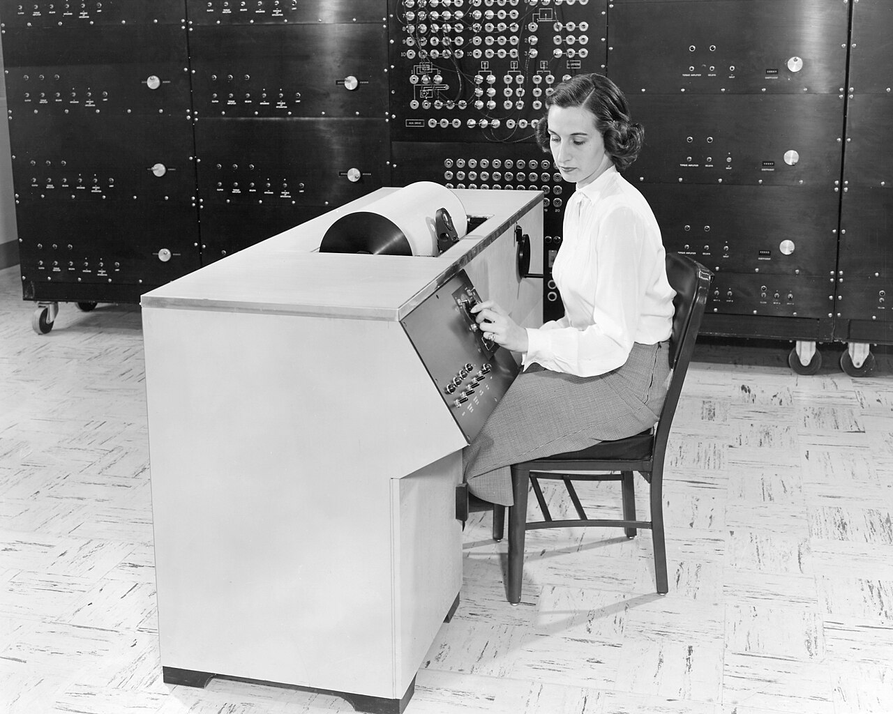
Computing With Physics
A digital computer counts. It represents a number as a string of discrete symbols and manipulates them with logic. An analog computer measures. It represents a number as a physical quantity that varies smoothly, a rotation, a current, a voltage, a fluid pressure, and it computes by arranging the physics so that the quantity you want falls out as a measurement.
The idea is old and intuitive. A slide rule multiplies by adding lengths (see Before the Computer: Mechanical Calculation). Lord Kelvin’s tide-predicting machine of 1872 used a chain running over a set of pulleys, each geared to one of the astronomical cycles that drive the tides, to sum their motions, and drew the prediction as a curve on a moving roll of paper. Kelvin’s brother James Thomson had designed a mechanical integrator, a wheel-and-disc mechanism that could compute the running total of a changing quantity. Kelvin saw that if you could connect integrators together, you could solve differential equations, the equations that describe almost everything that moves or changes in physics and engineering. He could not make the connection work: a single integrator’s output was too weak to drive the next one.
The strength of an analog computer is that the answer arrives at the speed of physics, all at once, no matter how complex the equation. Its weakness is equally built in: the answer is only as accurate as you can build and measure the hardware. A gear has backlash; a voltage has noise. Three or four digits of precision was typical, and getting a fifth was expensive. A digital computer, by contrast, buys precision cheaply: add more bits.
From Kelvin to Bush
The problem Kelvin could not solve, torque amplification, was solved at MIT. Between 1928 and 1931 Vannevar Bush and Harold Hazen built the first practical general-purpose differential analyzer, a room-sized assembly of rotating shafts, gears, and six mechanical integrators, with a torque amplifier on each integrator so its output could drive the next stage (see Vannevar Bush and the Memex). An operator set up a problem by physically connecting shafts with gears and chains to match the terms of a differential equation, a process that could take days. Then the machine ran the equation and plotted the solution.
Through the 1930s the differential analyzer was the standard machine for solving differential equations, and copies and variants spread. Douglas Hartree and Arthur Porter built a model at Manchester in 1934, largely out of Meccano parts, to prove the design cheaply; a full-scale machine followed in 1935. The Oslo analyzer of 1938 had twelve integrators. The most consequential copy was at the Moore School of Electrical Engineering at the University of Pennsylvania, where the US Army used it through the early 1940s to compute artillery firing tables, the same backlog of calculation that would justify building ENIAC on the same site. ENIAC was digital, and it was built in part because the differential analyzer, for all its speed, could not keep up with wartime demand and had to be re-geared by hand for every new problem.
The Rocket That Computed Its Own Flight
The machines described so far were mechanical and stationary. The leap to electronics came from a German engineer solving a problem no gear train could fit inside: how to make a rocket steer itself in flight.
Helmut Hölzer (born 27 February 1912, died 19 August 1996) had the idea as a student. In 1935 at the Technische Hochschule Darmstadt, a novice glider pilot who wanted to measure his own ground speed, he reasoned that electrical circuits could perform integration and differentiation on the fly. His professors talked him out of it as a student project. At Peenemünde, working under Wernher von Braun on the A-4 rocket that became the V-2, he built it. In early 1942 Hölzer assembled a fully electronic analog computer, using vacuum-tube circuits to do the integration, to simulate and test the rocket’s flight dynamics on the ground. It is widely credited as the first fully electronic analog computer.
The same principle then flew. The Mischgerät (“mixing device”), the V-2’s onboard guidance computer, was an electronic analog circuit that took the outputs of the rocket’s gyroscopes, computed the corrections needed to keep the vehicle stable and on its programmed trajectory, and drove the graphite vanes in the exhaust that steered it. It was an embedded analog control computer riding a ballistic missile in 1944, solving the guidance equation continuously in real time because there was no other way to do it fast enough. After the war Hölzer came to the United States with the von Braun group under Operation Paperclip, worked at Fort Bliss and Redstone Arsenal, and rose to Director of the Computation Division at NASA’s Marshall Space Flight Center, where analog and hybrid computers simulated the Saturn rockets before they were built.
The Electronic Analog Era
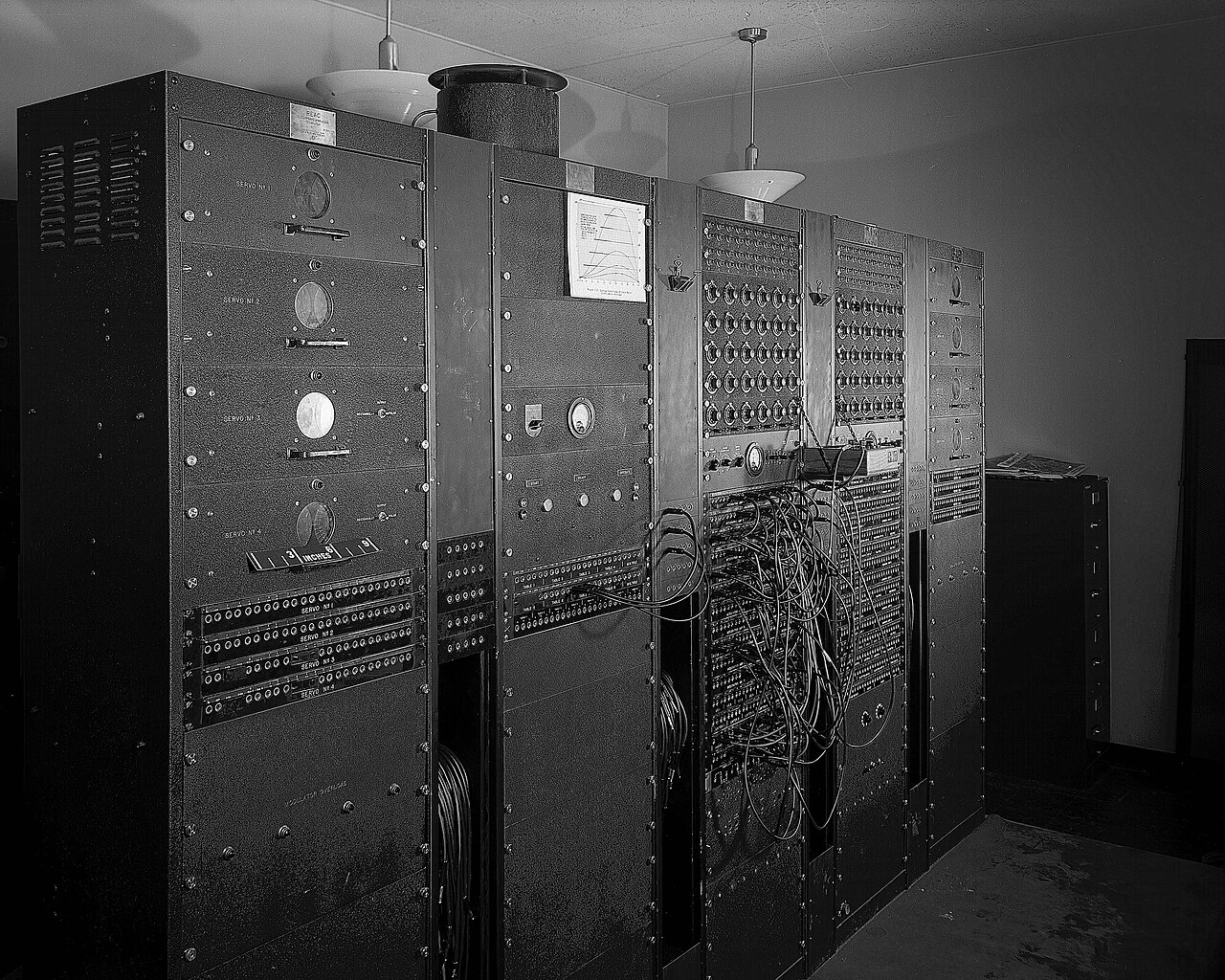
Hölzer’s insight, that a high-gain amplifier with a capacitor in its feedback path integrates its input, became the basis of a whole industry once a suitable amplifier existed. The operational amplifier, named in a 1947 paper by John Ragazzini, Robert Randall, and Frederick Russell and cheap once transistors arrived, was named for exactly this use: performing mathematical operations. With op-amps you could build integrators, summers, and multipliers, wire them together on a patch panel, set coefficients with precision potentiometers, and have a differential equation solved as fast as the electronics could settle, thousands of times a second.
Through the 1950s and 1960s the electronic analog computer was the standard tool for simulation. If you wanted to know how an aircraft would handle, how a missile would fly, how a chemical plant or a power grid or a nuclear reactor would respond before you built it, you modeled it on an analog computer and watched the answer on an oscilloscope in real time. Electronic Associates (EAI) of West Long Branch, New Jersey, dominated the market; its 231R had twenty integrators and vacuum tubes and simulated Project Mercury, Gemini, and the X-15, and its later solid-state 8800 had sixty-four. NASA, Lockheed, Martin Marietta, Hughes, and their European counterparts ran dedicated analog computing centers. The flight simulators that trained the first astronauts were analog. For real-time dynamics in the aerospace age, nothing digital was fast enough yet.
Why Digital Won
The analog computer had two permanent disadvantages, and digital technology attacked both at once. The first was precision. An analog machine’s accuracy is limited by the quality of its components and the noise in its signals; three or four significant figures was normal, and each additional digit cost real money in better parts. A digital computer reaches any precision you want by adding bits, at trivial marginal cost. The second was programming. Setting up an analog computer meant physically wiring a patch panel and turning coefficient dials, a slow, error-prone, problem-specific process. A digital computer is reprogrammed by loading different software.
For a while the answer was to combine the two. Hybrid computers of the 1960s used an analog section for the fast, continuous integration and a digital section for precision, logic, and control, joined by analog-to-digital and digital-to-analog converters. It was a genuine engineering compromise, and it kept analog techniques alive in flight simulation and process control into the 1970s.
Then the compromise stopped being worth it. The integrated circuit made digital computation cheaper every year, on the curve of Moore’s Law; digital machines got fast enough to simulate dynamic systems in real time, and they came with arbitrary precision and reprogrammability for free. The analog computer had no such curve to ride. By the mid-1970s it had lost its last strongholds, and by the 1980s it was a subject for computing museums. It is the clearest kind of dead end: not a bad idea, but a good idea overtaken by a technology that scaled and one that did not.
The Analog Revival
The reason analog computing is back is the same reason it was good in the first place: some operations that cost a digital chip dearly are nearly free in analog. The dominant computation in a neural network is the multiply-and-accumulate, multiplying many inputs by many weights and summing the results. A digital processor does this one number at a time with millions of transistors switching, burning power mostly to move data between memory and the arithmetic unit. An analog circuit can do the whole multiply-and-sum in one physical step: encode the weights as the conductance of a grid of memory cells, apply the inputs as voltages, and the currents add up according to Ohm’s and Kirchhoff’s laws. The answer appears where the wires meet.
That is analog in-memory computing, and it is being built. The startup Mythic ships an Analog Matrix Processor that stores neural-network weights in NOR flash cells and does inference in the analog domain, claiming up to 25 trillion operations per second in a 3-watt power envelope, performance comparable to an embedded GPU at a tenth of the power. In 2023 IBM Research reported an analog AI chip with 35 million phase-change-memory devices reaching up to 12.4 trillion operations per second per watt, matching digital accuracy on a speech task while using far less energy. The old weakness, limited precision, turns out not to matter for neural-network inference, which tolerates noise well; the old strength, doing arithmetic in physics, is exactly what a power-constrained data center or a battery-powered device wants.
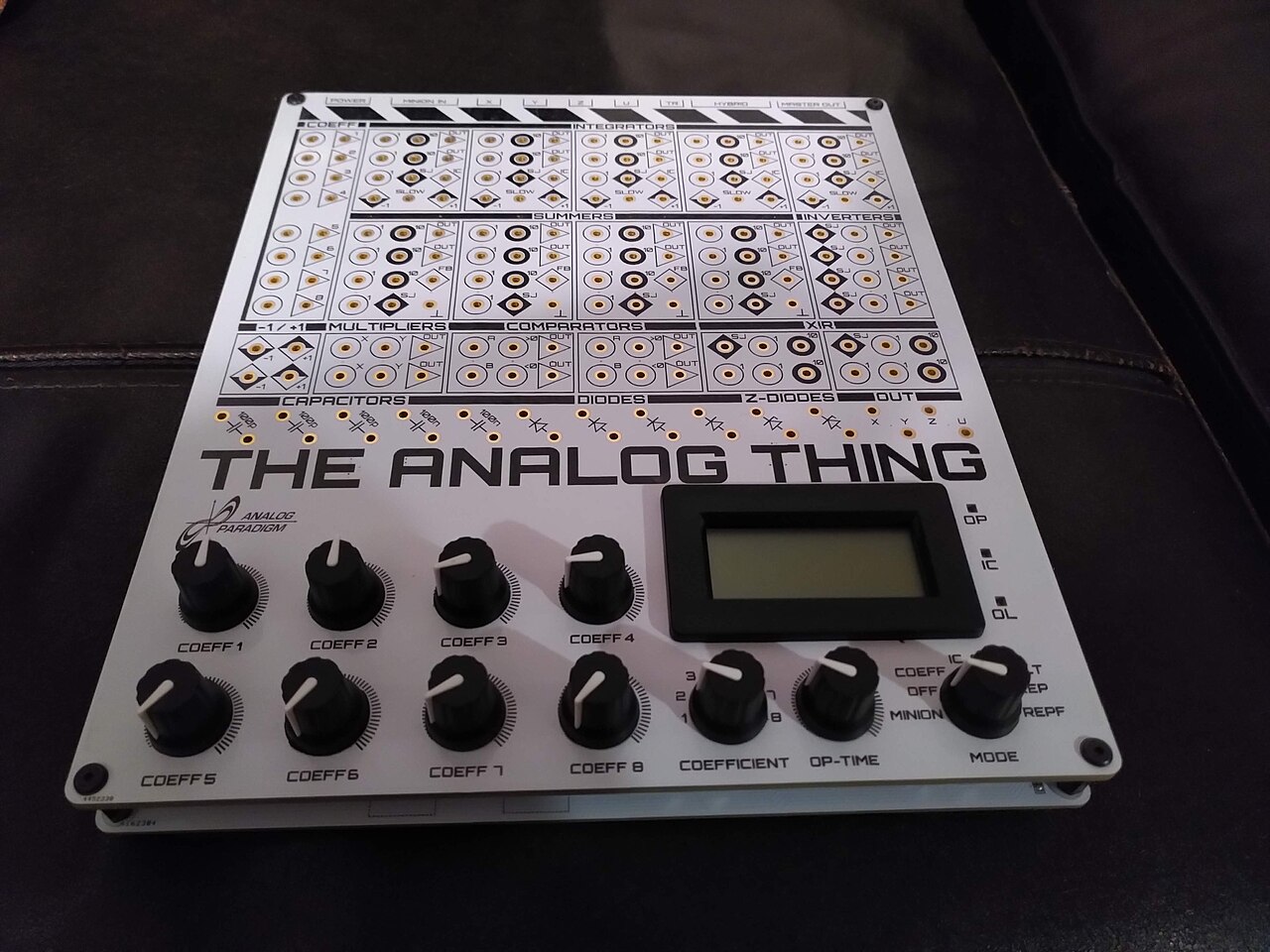
There is also a revival of the general-purpose analog computer, led from Germany by Bernd Ulmann, who runs a private analog-computer museum in Bad Schwalbach and co-founded anabrid in 2020 with the goal of putting an analog computer on a chip. In 2021 anabrid released THE ANALOG THING (THAT), a low-cost open-hardware analog computer for teaching and experiment. The pitch is not nostalgia but energy: as digital computing’s power demands keep climbing, doing part of the work in continuous physics is a way to compute more per joule. The machine that lost the twentieth century is being asked back for a problem the winner made worse.
A different kind of dead end
Most entries in this encyclopedia’s “dead end” tradition are technologies that failed on their merits or were killed by a rival that did the same job better. Analog computing is the rarer case of a sound idea beaten by a scaling law rather than a flaw, and then invited back decades later when the scaling law that beat it, digital’s appetite for power, became the problem. The history is worth keeping straight: analog did not fail, it was outrun, and the race is being re-run on different ground.
📚 Sources
- Differential analyser — Wikipedia (Kelvin/Thomson, Bush 1931, Hartree/Manchester, Moore School)
- Analog computer — Wikipedia (op-amps, EAI, hybrid computers, VLSI and neuromorphic revival)
- Helmut Hölzer — Wikipedia (biography, dates, Peenemünde, NASA Marshall)
- “Nachruf Dr.-Ing. Helmut Hoelzer”, RZ-Mitteilungen 13, Humboldt-Universität zu Berlin, January 1997 (death on 19 August 1996)
- Mischgerät (V-2 guidance computer) — Wikipedia
- James E. Tomayko, “Helmut Hoelzer’s Fully Electronic Analog Computer”, IEEE Annals of the History of Computing 7(3), 1985 — doi:10.1109/MAHC.1985.10025
- New analog AI chip design uses much less power for AI tasks — IBM Research (2023 phase-change-memory speech chip, 35 million PCM devices, 12.4 TOPS/W)
- An analog-AI chip for energy-efficient speech recognition and transcription — Nature (IBM, 2023)
- Mythic M1076 Analog Matrix Processor — Mythic (NOR-flash analog inference, up to 25 TOPS at about 3 W)
- Bernd Ulmann, Analog Computing, De Gruyter — publisher page
- THE ANALOG THING / anabrid — anabrid (THAT, analog computing for the 21st century)
- Electronic Associates — Wikipedia (West Long Branch, 231R and 8800, Mercury/Gemini/X-15 simulation)
- John R. Ragazzini, Robert H. Randall, Frederick A. Russell, “Analysis of Problems in Dynamics by Electronic Circuits”, Proceedings of the IRE 35(5), 1947, pp. 444–452 — doi:10.1109/JRPROC.1947.232616
- Tide-predicting machine — Wikipedia (Kelvin’s 1872 machine, chain over pulleys, pen on moving paper)
- Bernd Ulmann — Wikipedia (German; anabrid founded 2020, collection in Bad Schwalbach)
- Image: THE ANALOG THING.jpg by Jwdietrich2 (CC BY 4.0), via Wikimedia Commons